Numpy

NumPy is a Python library used for working with arrays, linear algebra, fourier transform, and matrices. NumPy stands for Numerical Python and it is an open source project. The array object in NumPy is called ndarray, it provides a lot of supporting functions that make working with ndarray very easy.

Arrays are very frequently used in data science, where speed and resources are very important.

  • We’ve already installed numpy into our virtual environment in other pages so we just need to import it into Python
  • After we load reticulate
library(reticulate)
py_install("numpy")
Using virtual environment "~/.virtualenvs/r-reticulate" ...
py_install("matplotlib")
Using virtual environment "~/.virtualenvs/r-reticulate" ...
import numpy as np
import matplotlib.pyplot as plt

np.array


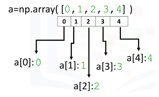
Each element in an array is of the same type:
Cast np.array

Note: ([ ]) the parenthesis and brackets

a = np.array([7,5,2,3,4])
a
array([7, 5, 2, 3, 4])

Select

Just like a list, and similar to df, and dictionaries we can access each element by their location

a[1]
np.int64(5)

Type

type(a)
<class 'numpy.ndarray'>

dtype

a.dtype
dtype('int64')

Assign value

  • Single value: Of course we can edit existing values by assignment.
a[2] =14
a
array([ 7,  5, 14,  3,  4])
  • Multiple values: let’s assign the 4th and 5th elements new values
a[3:5] = 104, 658
a
array([  7,   5,  14, 104, 658])

Slicing

a[0:3]
array([ 7,  5, 14])

Step Slicing

  • If we want every other element in a slice
  • If we don’t pass it an integer it will default to 1
a[0:5:2]
array([  7,  14, 658])

Till End

  • If we don’t pass an end to the slice it will consider proceed till the end
  • This is useful when we don’t know how long the array is (not sure how that could happen?)
  • This will slice from the 3rd element till the end
a[2:]
array([ 14, 104, 658])

Slice with List

  • First create the list
  • Then use list in the brackets
list = [0,3,4]
a[list]
array([  7, 104, 658])

Size

  • Size is the number of elements in the arrary
a.size
5

Ndim

  • The number of array dimensions, or the rank. Of course it should be 1, it will be used when we get to vectors
a.ndim
1

Shape

a.shape
(5,)

Statistical Functions


Mean

a.mean()
np.float64(157.6)

Std

a.std()
np.float64(252.9273413452962)

Max

a.max()
np.int64(658)

Min

a.min()
np.int64(5)

Sum

a.max()+ a.min()
np.int64(663)

Operations


You can use arithmetic operators on numpy arrays:

Add

u = np.array([1,0])
v = np.array([0,1])
z = np.add(u,v)
z
array([1, 1])

You can visualize the operation like this

import time 
import sys

def Plotvec1(u, z, v):
    
    ax = plt.axes()              # to generate the full window axes
    ax.arrow(0, 0, *u, head_width=0.05, color='r', head_length=0.1)
    # Add an arrow to the  U Axes with arrow head width 0.05, color red and arrow head length 0.1
    plt.text(*(u + 0.1), 'u')    # Adds the text u to the Axes 
    
    ax.arrow(0, 0, *v, head_width=0.05, color='b', head_length=0.1)
    # Add an arrow to the  v Axes with arrow head width 0.05, color red and arrow head length 0.1
    plt.text(*(v + 0.1), 'v')    #Adds the text v to the Axes 
    
    ax.arrow(0, 0, *z, head_width=0.05, head_length=0.1)
    plt.text(*(z + 0.1), 'z')   #Adds the text z to the Axes 
    plt.ylim(-2, 2)             #set the ylim to bottom(-2), top(2)
    plt.xlim(-2, 2)             #set the xlim to left(-2), right(2)
Plotvec1(u,z,v)

Example:

arr1 = np.array([10, 11, 12, 13, 14, 15])
arr2 = np.array([20, 21, 22, 23, 24, 25])
arr3 = np.add( arr1, arr2)
arr3
array([30, 32, 34, 36, 38, 40])

Subtract

arr4 = np.subtract( arr2, arr1)

Multiply

x = np.array([1,2,3])
y = np.array([4,5,6])
z = np.multiply(x,y)
x
array([1, 2, 3])
y
array([4, 5, 6])
z
array([ 4, 10, 18])

Divide

a = np.array([10,20,30])
b = np.array([1,2,3])
c = np.divide(a,b)
a
array([10, 20, 30])
b
array([1, 2, 3])
c
array([10., 10., 10.])

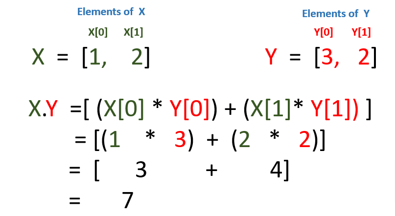
Dot Product

x = np.array([1,2])
y = np.array([3,2])
np.dot(x,y)
np.int64(7)

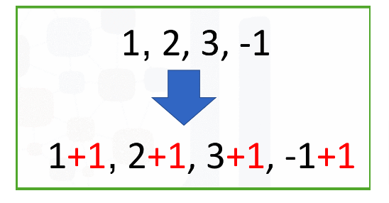
Add Constant

u = np.array([1,2,3,-1])
u + 1
array([2, 3, 4, 0])

Sine Function

  • Let’s say we want to apply the sine function to an arrary
x = np.array([0, np.pi/2, np.pi])
y = np.sin(x)

Linspace

  • Linspace returns evenly spaced numbers over a specified interval
  • Syntax: numpy.linspace(start, stop, num = int value)
  • Let’s say we want 5 evenly spaced numbers over the interval from -2 to 2
# Five evenly spaced numbers between -2 & 2
np.linspace(-2, 2, num=5)
array([-2., -1.,  0.,  1.,  2.])
# Nine evenly spaced numbers between -2 & 2
np.linspace(-2, 2, num=9)
array([-2. , -1.5, -1. , -0.5,  0. ,  0.5,  1. ,  1.5,  2. ])
# Make an array from 0 to 2pi with 100 elements
w = np.linspace(0, 2*np.pi, num=100)

# Calculate the sine function to each element in the w array
y = np.sin(w)

# Plot the result
plt.plot(w, y)

Vectors


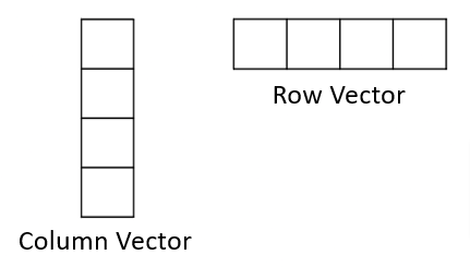
A 1D array is often termed a vector. Depending on the orientation of the data, it could be a row vector or a column vector
Add/Subtract

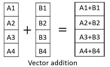
You can add or subtract two vectors by going across:
Multiply

The same apply, just multiply across.

Note all these operations require both to have the same size

Add/Subtract/X Constant

Here the same applies, the constant is added, subtracted, or multiplied to or from each element

Matrices


A 2D array is called a matrix. They are called rectangular arrays. The operations above apply to these as well in the same fashion.

Dot product follows a different rule:
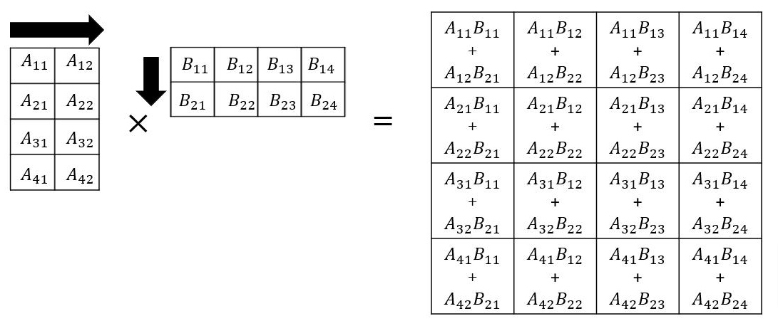
  • Both have to have the same shape, meaning if one is 2x4(2 col x 4 rows) the other should be 4x2(4 col, 2 rows)
  • The result will be a 4x4 matrix

  • If the configuration is reversed where we have a 4x2 to be multiplied with a 2x4 we end up with a 2x2 matrix

Create 2D array

Create List

import numpy as np
# Create a list
a = [[11, 12, 13], [21, 22, 23], [31, 32, 33]]
a
[[11, 12, 13], [21, 22, 23], [31, 32, 33]]

Convert List to Array

A = np.array(a)
A
array([[11, 12, 13],
       [21, 22, 23],
       [31, 32, 33]])
A.ndim
2
A.shape
(3, 3)
A.size
9

Select

As before we can use [] to access different elements of the array.
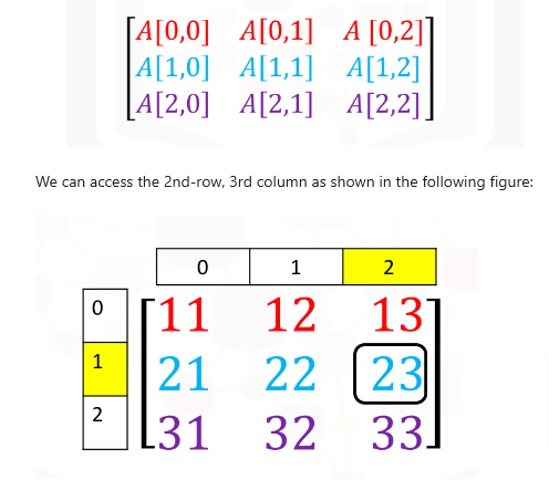
# Access element on the second row and 3rd column
a = [[11, 12, 13], [21, 22, 23], [31, 32, 33]]
A = np.array(a)
A[1,2]
np.int64(23)
# or we can use
A[1][2]
np.int64(23)

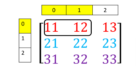
Slice

A[0, 0:2]
array([11, 12])

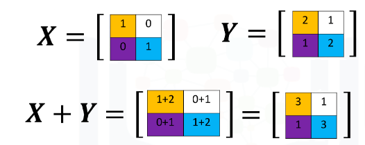
Add

X = np.array([[1, 0], [0, 1]]) 
Y = np.array([[2, 1], [1, 2]]) 
Z = X + Y

Multiply X Constant

Z * 2
array([[6, 2],
       [2, 6]])

Hadamard product

Multiplication of two arrays corresponds to an element-wise product Hadamard product. Therefore you multiply each of the elements in the same position.
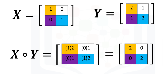
X = np.array([[1, 0], [0, 1]]) 
Y = np.array([[2, 1], [1, 2]]) 
X * Y
array([[2, 0],
       [0, 2]])
  • Or we can do it with the dot product
# Create two matrices
A = np.array([[0, 1, 1], [1, 0, 1]])
B = np.array([[1, 1], [1, 1], [-1, 1]])
A
array([[0, 1, 1],
       [1, 0, 1]])
B
array([[ 1,  1],
       [ 1,  1],
       [-1,  1]])

Dot Product

Z = np.dot(A,B)
Z
array([[0, 2],
       [0, 2]])

Reference


Here’s a list of operations that can be performed using Numpy

Operation Description Example
Array Creation Creating a NumPy array. arr = np.array([1, 2, 3, 4, 5])
Element-Wise Arithmetic Element-wise addition, subtraction, and so on. result = arr1 + arr2
Scalar Arithmetic Scalar addition, subtraction, and so on. result = arr * 2
Element-Wise Functions Applying functions to each element. result = np.sqrt(arr)
Sum and Mean Calculating the sum and mean of an array.Calculating the sum and mean of an array. total = np.sum(arr)<br>average = np.mean(arr)
Maximum and Minimum Values Finding the maximum and minimum values. max_val = np.max(arr)<br>min_val = np.min(arr)
Reshaping Changing the shape of an array. reshaped_arr = arr.reshape(2, 3)
Transposition Transposing a multi-dimensional array. transposed_arr = arr.T
Matrix Multiplication Performing matrix multiplication. result = np.dot(matrix1, matrix2)
a=np.array([0,1]) 

b=np.array([1,0]) 

np.dot(a,b) 
np.int64(0)
a*b
array([0, 0])
X=np.array([[1,0,1],[2,2,2]]) 

X
array([[1, 0, 1],
       [2, 2, 2]])
out=X[0:2,2]
out
array([1, 2])
X=np.array([[1,0],[0,1]]) 

Y=np.array([[2,1],[1,2]]) 

Z=np.dot(X,Y) 
X
array([[1, 0],
       [0, 1]])
Y
array([[2, 1],
       [1, 2]])
Z
array([[2, 1],
       [1, 2]])